Table of Contents
The simplex algorithm is used in mathematics to solve linear optimization problems, or so-called linear programs. In an economic context, the simplex method is used, for example, to calculate cost minimization or profit maximization while adhering to certain constraints.
Since it is an iterative process, finding the optimal solution takes place in several steps. The process begins with a feasible basic solution, which is then checked for optimality. If the basic solution is not optimal, a new, improved solution is sought, which is then checked for optimality. The process ends once an optimal solution has been found.
In the simplest case, the problem already exists as a standard linear programming problem, i.e., a general maximization problem with constraints. If this is not the case, the problem can be transformed into one using simple arithmetic operations.
Transformations
Example:
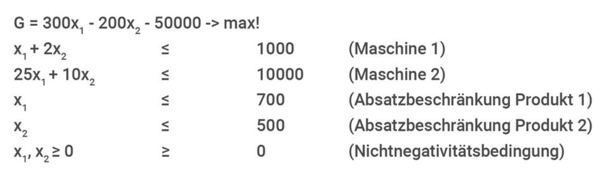
A firm produces goods 1 and 2 using two existing machines. Machine 1 has a capacity of 1,000 minutes, and machine 2 has a capacity of 10,000 minutes. Good 1 requires one minute of runtime on machine 1 and 25 minutes on machine 2. Good 2, on the other hand, requires 2 minutes on machine 1 but only 10 minutes on machine 2. Since the market is relatively small, no more than 700 units of good 1 and 500 units of good 2 can be sold. The firm's profit function is: G = 300 x 1 + 200 x 2 – 50,000.
How much of each good should the firm produce if it wants to maximize profit, subject to all constraints?
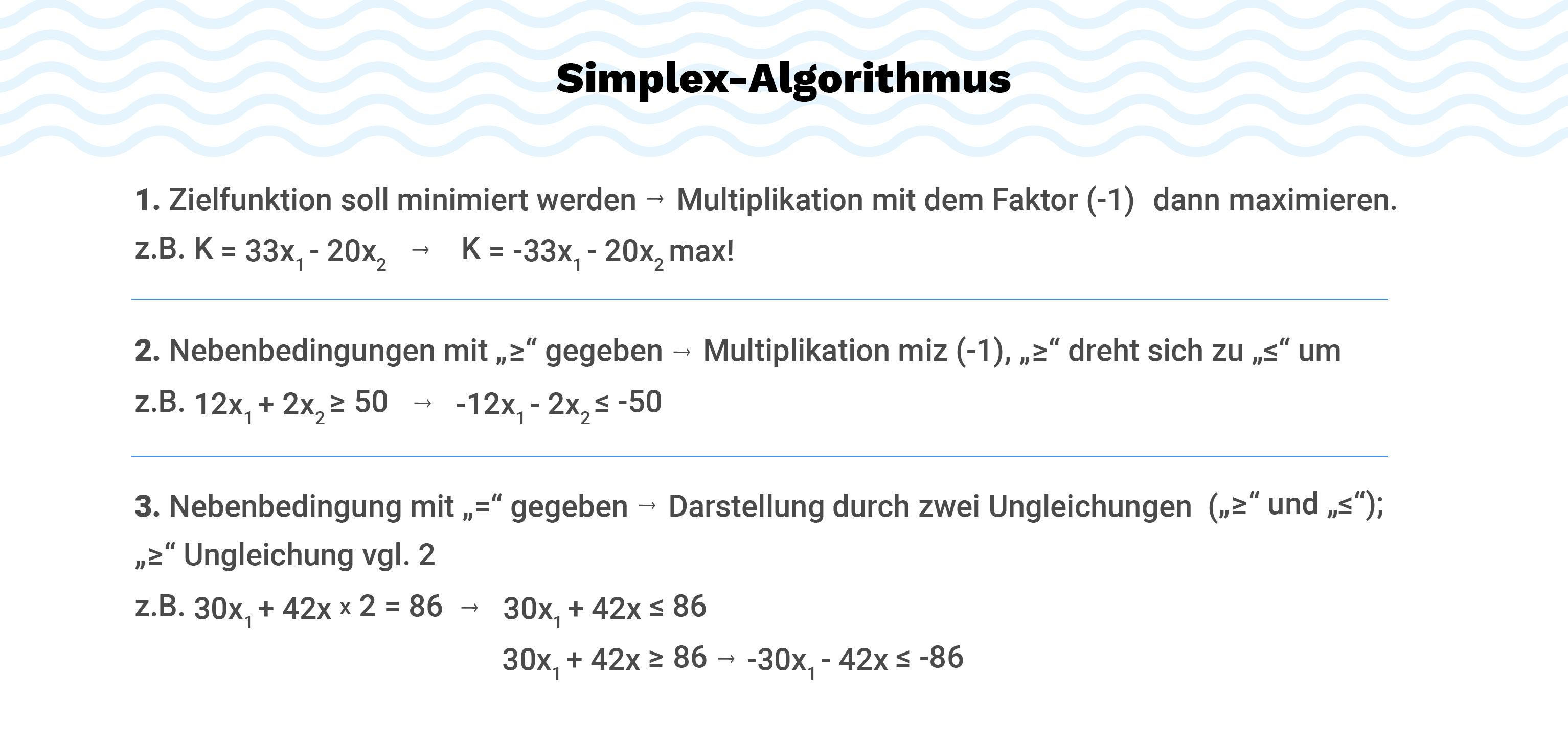
To apply the Simplex algorithm, the inequalities of the constraints must be transformed into a system of equations. This is done using so-called slack variables, which represent unused capacity in the system of equations. Furthermore, the objective function must be converted into the form "... = constant" without making the objective function value negative.

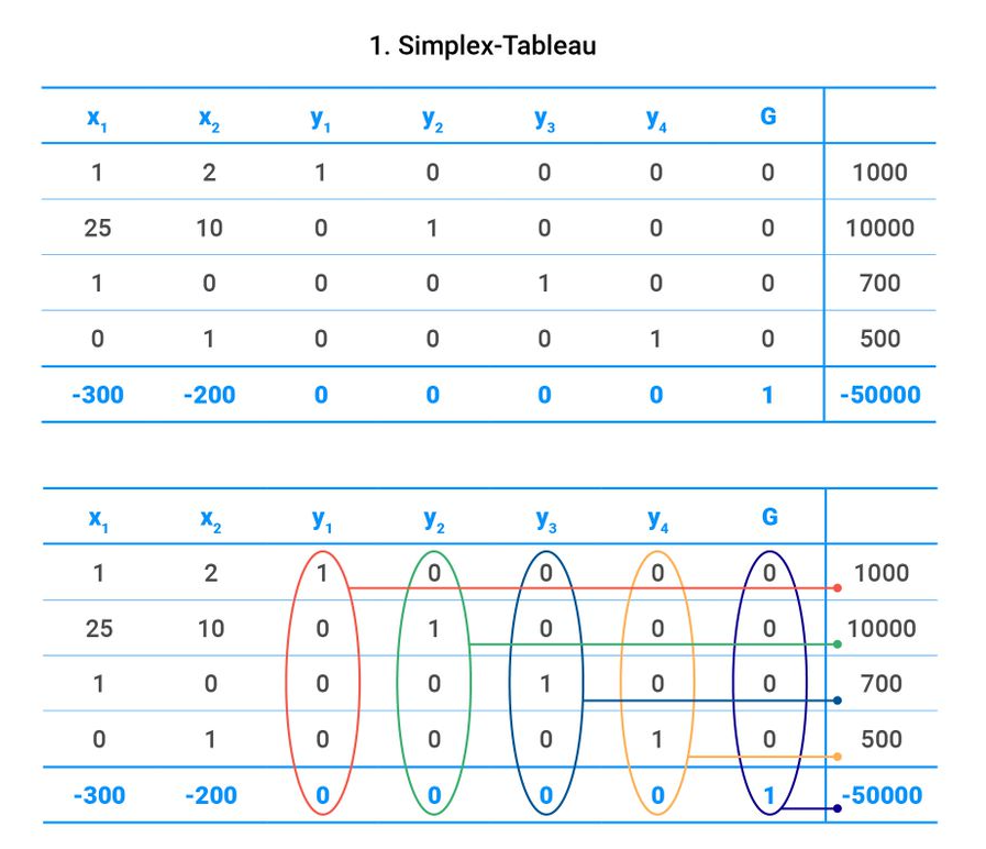
If the constraints are in equation form, all the coefficients of the problem can be transferred to a so-called simplex table. Each variable has its own column, and each constraint has its own row. The objective function is entered in the bottom row.
The first basic solution can then be read from the first simplex table. To do this, each variable that has a unit vector below it is assigned the value from the last column that is on the same level as the "1" in the unit vector. If a variable has no unit vector below it, the variable is assigned the value 0.
The solution is not optimal as long as there is a negative value in the objective function row (=last column of the table). To do this, a unit vector must be generated using row operations in the column where the value of the objective function row is smallest. The column with the smallest value is then called the pivot column.
To determine the position of the "1" of the unit vector, the so-called pivot row must first be found. This is located at the point where the quotient of the respective element of the pivot column and the last column of the table is smallest. Negative and indeterminate (e.g., 120) quotients are not considered. The element that is located in both the pivot column and the pivot row is called the pivot element; the "1" of the unit vector is then generated at this point.
The pivot element cannot be in the bottom row or the last column.

Note:
The solution is not optimal as long as the objective function row contains a negative value! The algorithm only ends when the optimal solution has been found.
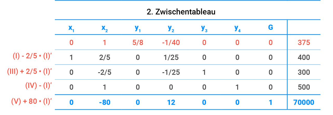
To find a better solution, row operations are used to try to make the pivot element a "1" and the remaining elements in the column a "0". For better clarity, an intermediate table can be created. This table differs from the previous simplex table in that a first row operation has already taken place in the pivot row. Using this modified row, the remaining rows are then adjusted so that a unit vector is generated in the pivot column. Once this has been generated, the second simplex table is available, from which the improved solution can be read off.
Continuation Example:
The pivot element in this example was the element "25," which should now become the "1" of the unit vector. To do this, the entire second row is multiplied by 125. The new second row is then referred to as (II).


Improved basic solution: x1 = 400; x2 = 600; y2 = 0; ys = 300; y4 = 500; G = 70000
→ Current solution not yet optimal, continue the algorithm!

→ Optimal table = end of the simplex algorithm
Optimal solution: x1* = 250; x2* = 375; y1* = 0; y2* = 0; y3* = 450; y4* = 125; G* = 100,000
Interpretation: The company achieves maximum profit of 100,000 when it produces 250 units of Good 1 and 375 units of Good 2. Both Machine 1 and Machine 2 are fully utilized. There is an unused sales potential of 450 units of Good 1 and 125 units of Good 2.


